Large language models make text generation look deceptively simple: a prompt goes in, a probability distribution comes out, and one token is added at a time. Inside the model, however, each token passes through many transformer blocks, and most of the learned parameters live in their linear layers.
That makes the large weight matrices in those layers a natural target for compression. But useful pruning is not simply a matter of finding small numbers and replacing them with zeros. The real question is:
After several weights disappear, how should the surviving weights move together so that the layer’s output changes as little as possible?
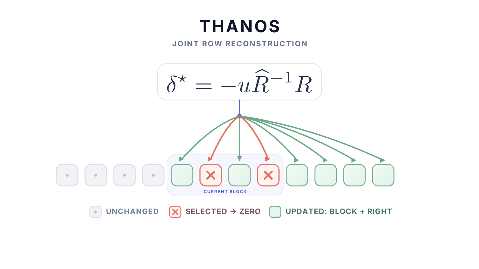
Thanos treats pruning as this coordinated reconstruction problem. It combines calibration data, second-order information, and a direct block-wise compensation rule. For unstructured sparsity, it also uses a dynamic global pruning budget.
The compression target: linear layers
A transformer block contains attention projections, feed-forward projections, normalization, residual connections, and nonlinearities. Architectures differ in their details, but the large learned matrices repeat throughout the model. Those matrices dominate parameter storage in the dense transformer families studied by this project.
Pruning sets selected entries of a matrix to zero:
- Unstructured sparsity allows zeros anywhere. It is flexible, but it needs suitable sparse storage and kernels before zeros translate into faster inference.
- Semi-structured sparsity constrains each small group of weights to retain exactly nonzero entries, such as 2:4 or 4:8. The constraint is less flexible, but it can align better with supported hardware paths.
In both cases, the mathematical task is the same: choose which weights to remove and reconstruct the rest.
The layer-reconstruction lens
Consider one linear layer. Let
- be its original weight matrix;
- contain calibration activations, with calibration examples arranged as columns;
- be the matrix after pruning and reconstruction; and
- be the change applied to the layer.
The original output is . A local pruning objective asks the new layer to reproduce it:
The Frobenius norm simply adds the squared error over all output coordinates and calibration examples. This objective is useful because it turns the vague instruction “preserve the model” into a concrete local reconstruction problem.
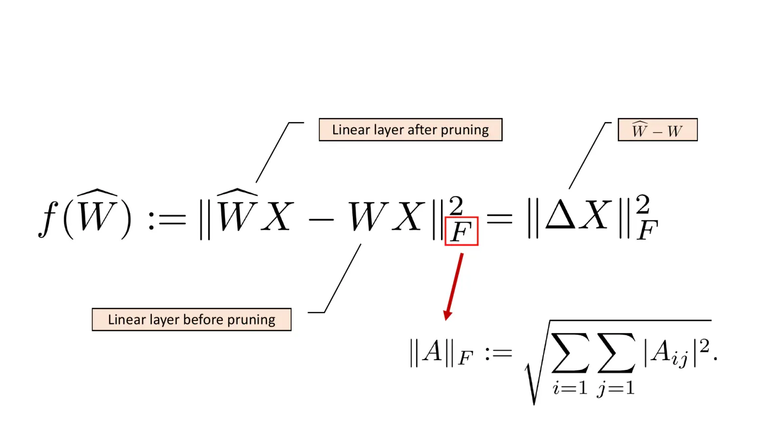
The loss also decomposes over the rows of :
That means each output row can be reconstructed independently. The rows share the same activation geometry, however, because they all receive the same . Efficient pruning algorithms are largely about exploiting that shared structure without creating a different expensive solve for every row and every mask.
Why magnitude alone misses important weights
The cheapest rule ranks weights by and removes the smallest. This ignores the feature that each weight multiplies.
Suppose we delete just and freeze every other value in row . The row update has one nonzero entry, , so the exact reconstruction error is
A small weight can therefore be important when its input feature is consistently active. Conversely, a larger weight may be relatively safe to remove when the corresponding feature is weak on the calibration data.
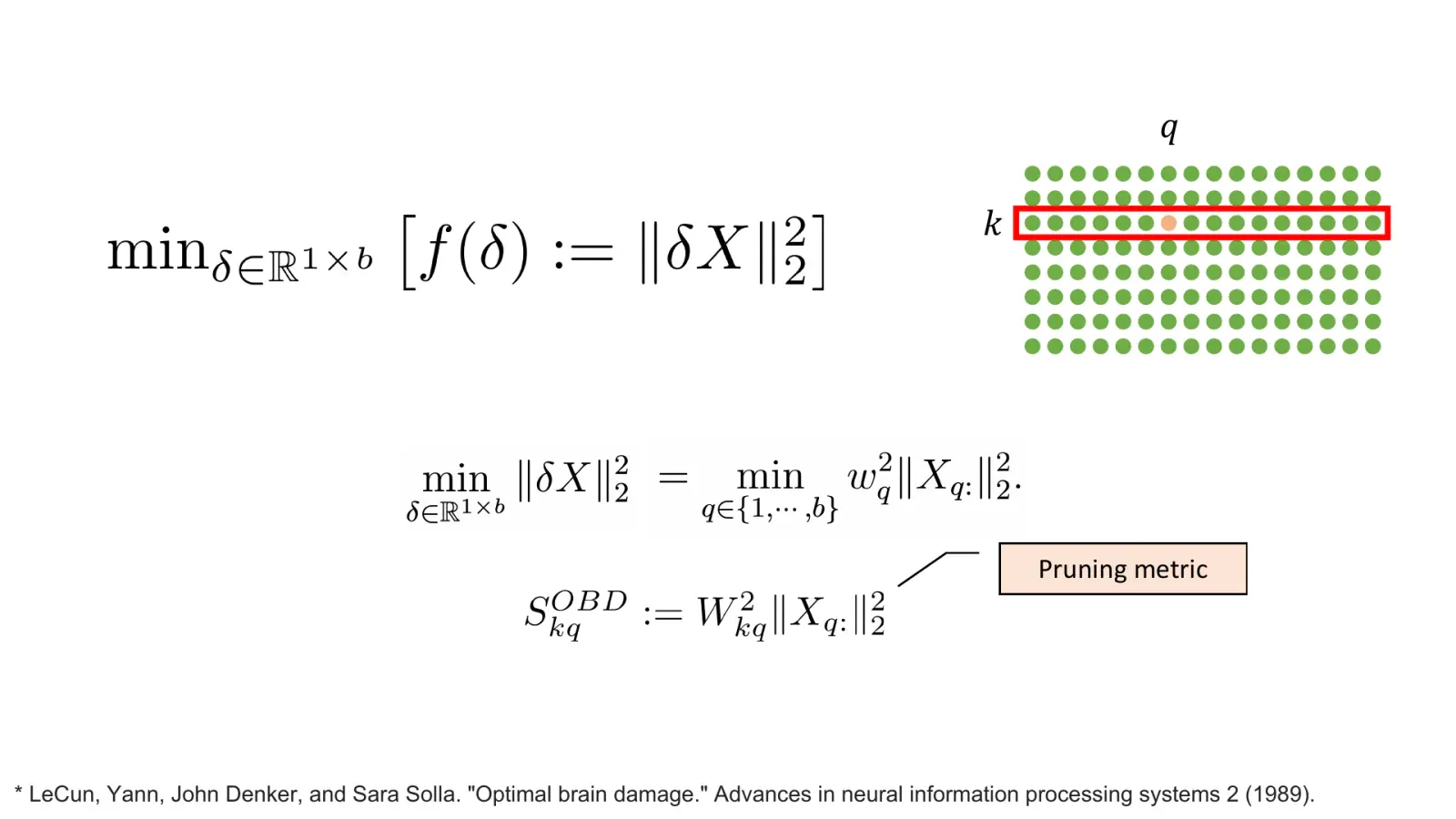
This Optimal Brain Damage-style view is also the intuition behind activation-aware methods such as Wanda, which ranks with . Squaring that expression gives the formula above without changing its ordering.
It is a better ranking signal than magnitude alone, but it still assumes that the retained weights cannot help.
One deletion with compensation: the OBS view
Now allow every coordinate in the row to change while forcing one chosen weight to zero. The activation Gram matrix is , which is the Hessian of the squared reconstruction loss up to a constant factor. Practical methods usually work with its damped form
where improves numerical stability. The off-diagonal entries encode correlations between input features. With , the solution below exactly minimizes the constrained reconstruction loss. With damping, it exactly minimizes the corresponding damped quadratic surrogate.
Optimal Brain Surgeon (OBS) solves the one-constraint problem in closed form. Using the inverse of , the compensating row update is
and the associated increase in the local reconstruction objective is proportional to
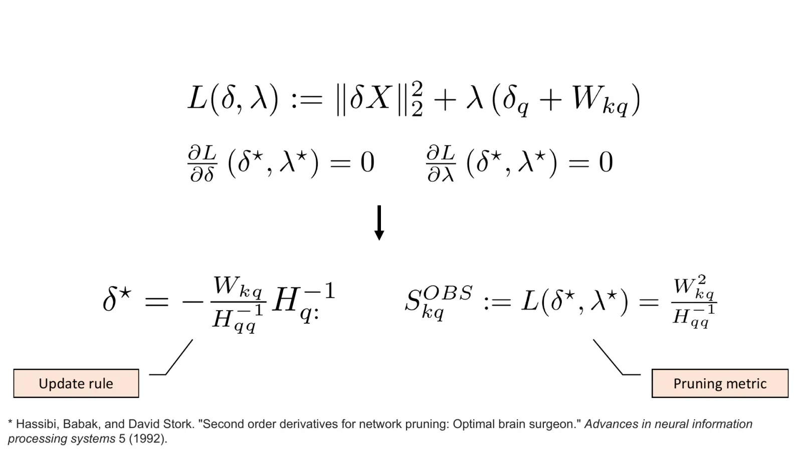
This is the important conceptual shift. Pruning is no longer only a mask-selection problem. It is also a reconstruction problem in which correlations decide how the error can be redistributed.
The scaling problem, and what SparseGPT changes
A direct row-wise application of OBS is impractical for a large layer. Different rows generally receive different masks. After every deletion, already-pruned coordinates must stay fixed, so each row would appear to need its own sequence of reduced systems.
SparseGPT made OBS-style reconstruction practical at LLM scale by synchronizing the work across rows:
- Process the matrix from left to right.
- Handle the current column for every row.
- Freeze that completed column for all rows at the same time.
- Propagate compensation only into columns that remain active.
- Refresh pruning decisions block by block as the unprocessed weights change.
Because every row retires the same column at the same time, the layer can share one sequence of reduced inverse-Hessian systems.
There is a subtle but important distinction here. Correctly conditioned sequential OBS can represent a fixed set of constraints; a direct joint solve is not evidence that sequential optimization is inherently incapable of doing so. The practical approximation in SparseGPT comes from the synchronized column schedule that makes systems reusable across rows.
Thanos starts from two design questions exposed by that schedule:
- Can the weights selected inside a manageable block be handled directly as one multi-constraint solve?
- Can a local block use information about the remaining global pruning budget, instead of being forced to match the same sparsity fraction as every other block?
Contribution one: solve a selected set directly
For one row, let be the coordinates selected for removal and let
collect their current values. From the inverse Hessian, take
Here, contains the rows associated with the selected coordinates, while is the small principal submatrix describing their interactions. The constrained optimum for the row update is
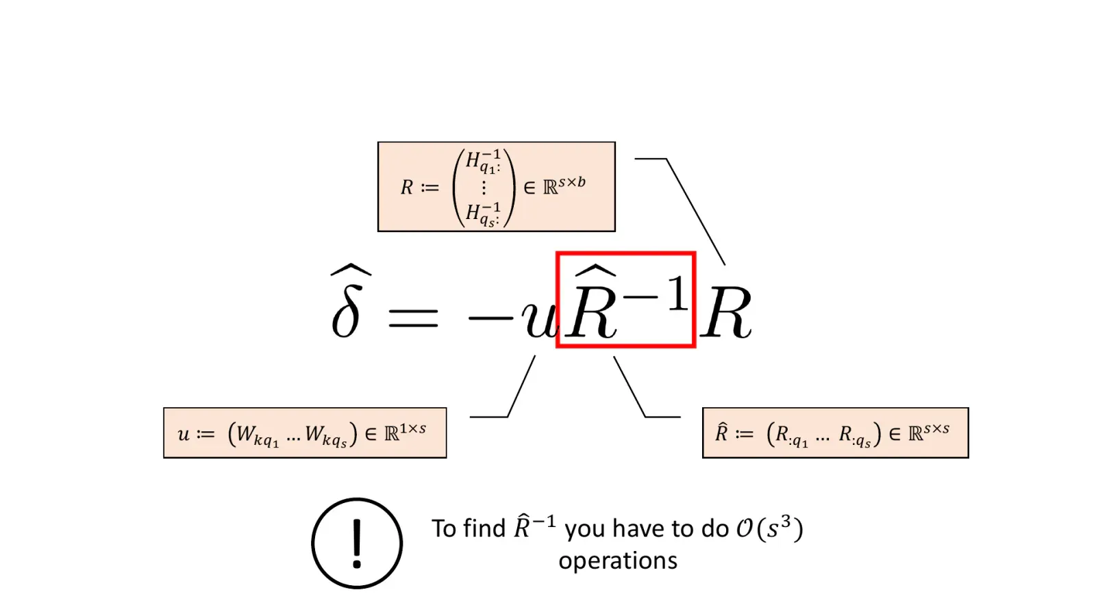
This update makes every coordinate in exactly zero and adjusts the retained coordinates to minimize the local quadratic model represented by . It is exact for the chosen set of deletions under that layer objective; it is not a claim of global optimality for the entire network.
Solving one system over the full layer would be too expensive. Thanos therefore works with manageable column blocks. Within a block, each row can remove several selected weights in one coupled update; the resulting compensation is propagated into the still-active part of the row.
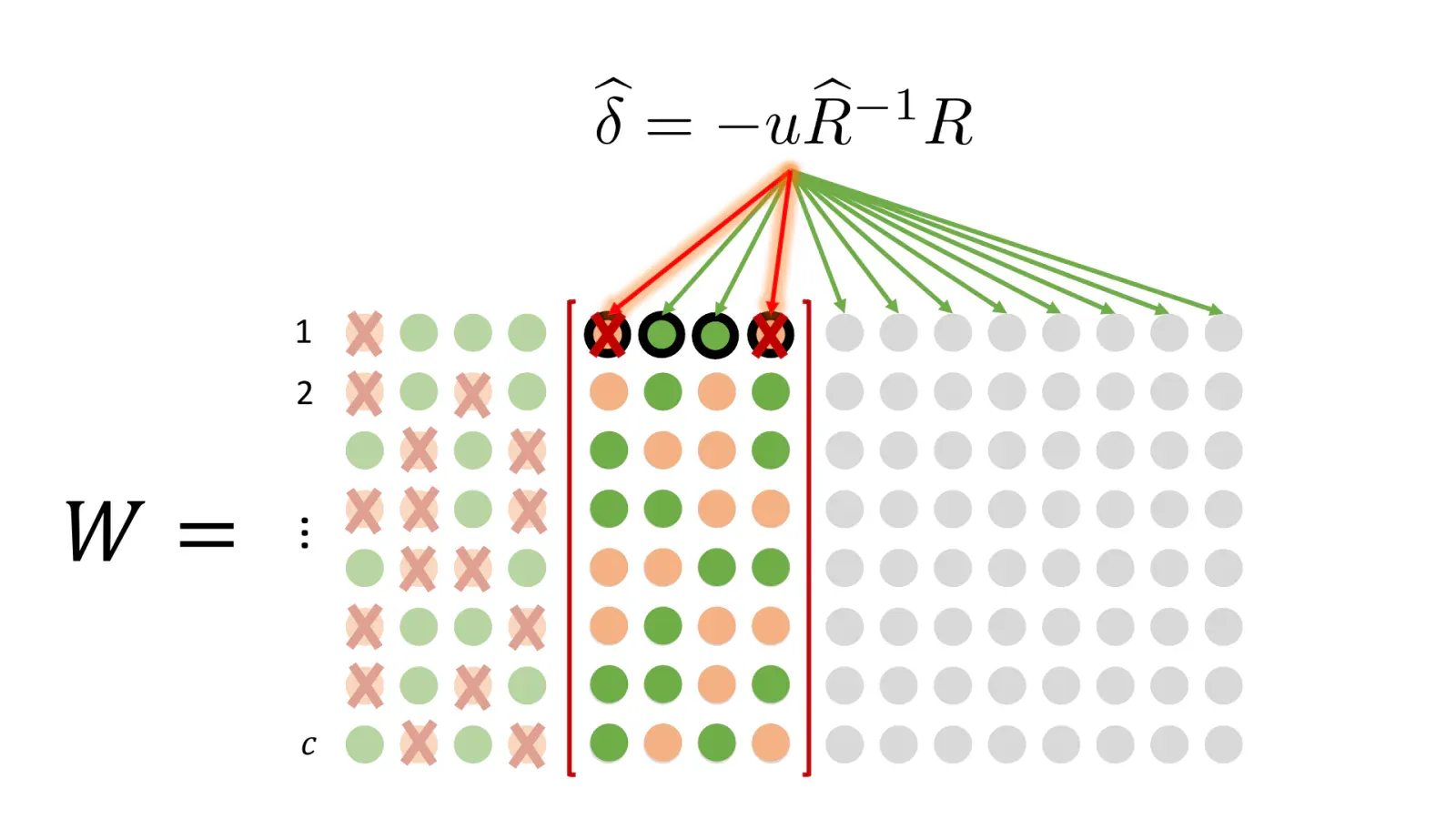
Block size is a real trade-off. Larger blocks expose more interactions to the joint solve, but they increase the size and cost of . Smaller blocks are cheaper but make the reconstruction more local.
Contribution two: keep the budget global and the execution local
A block-wise method still has to decide how many weights each block should lose.
Suppose the layer-wide target is 50% sparsity. Requiring every block to be exactly 50% sparse is stronger than necessary. One block may contain many low-impact weights, while the next may contain relatively important ones. Equal local quotas cannot move pruning capacity between them.
Computing one global mask at the beginning is not enough either: reconstruction changes the unprocessed weights, so their scores can become stale.
Thanos uses a dynamic residual budget:
- Count how many weights still need to be removed to reach the layer-wide target.
- Recompute activation-aware scores over the entire active region.
- Form a provisional global candidate set containing exactly that many lowest-scoring weights.
- Apply only the intersection of that candidate set with the current block.
- Perform the joint reconstruction, subtract the deletions from the residual budget, and repeat for the next block.
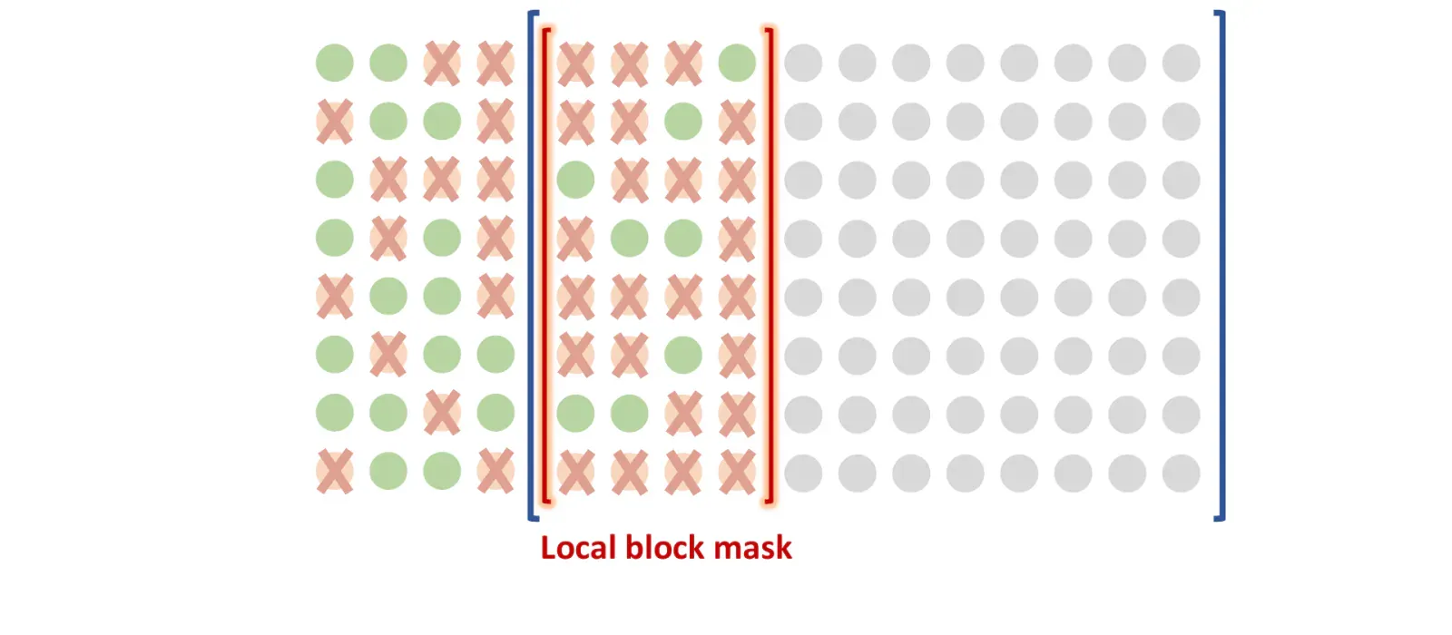
The mask stays responsive to changes caused by earlier reconstruction, yet the final number of zeros still meets the global target. Different blocks are free to receive different sparsity levels.
The semi-structured variant instead uses local, group-constrained masks. It retains the joint reconstruction step, but not the global residual-mask procedure described above.
Making irregular row masks batchable
Unstructured pruning introduces an implementation problem. In the same block, one row may select one weight, another two, and another three. Their vectors and interaction matrices then have different shapes, which prevents a straightforward batched solve.
Thanos pads every row to the maximum selected-set size in the batch:
- append zeros to ;
- append zero rows to ; and
- fill the unused part of with an identity matrix.
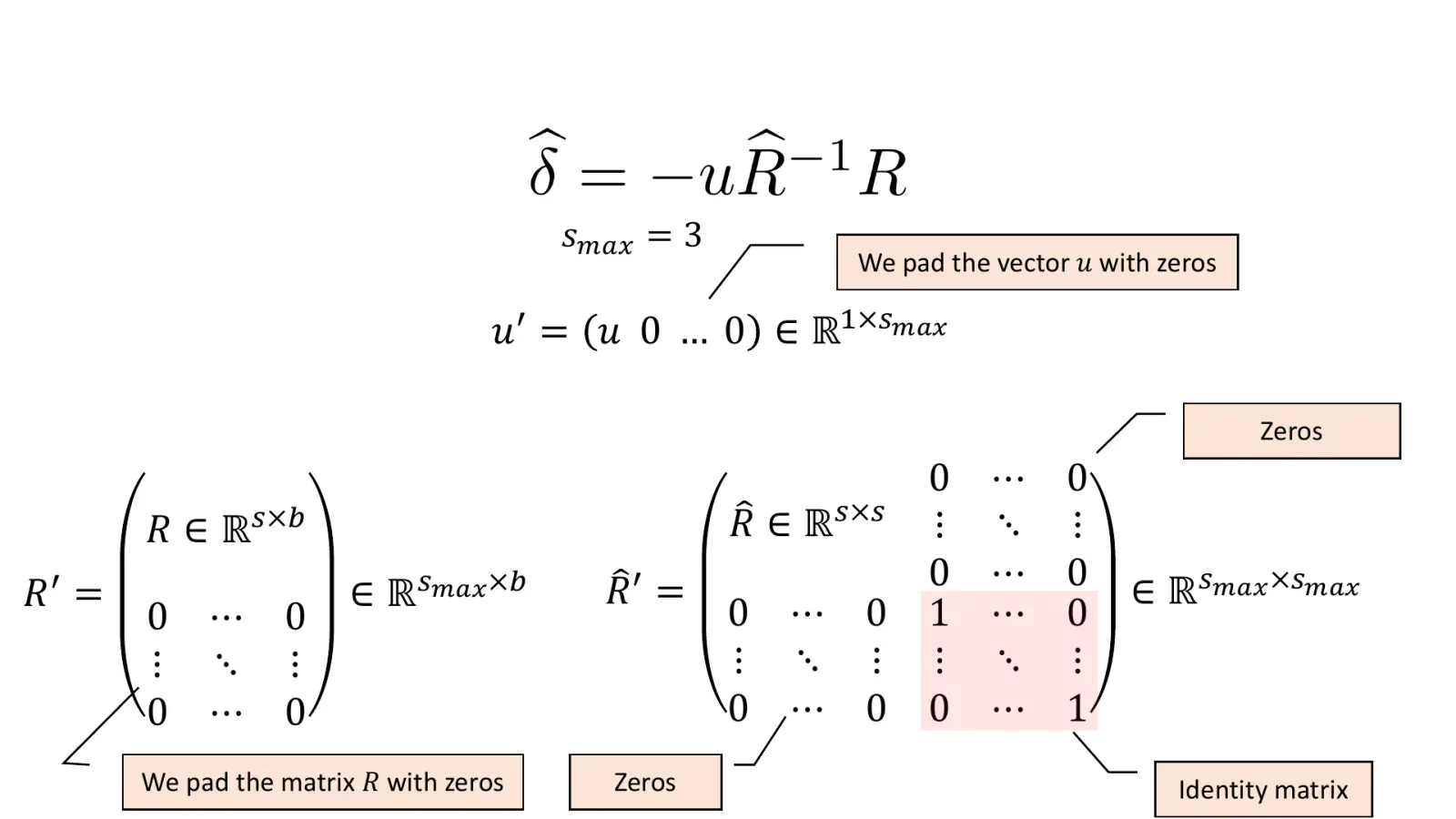
The dummy coordinates contribute no update, but the uniform shapes allow the row systems to run through batched PyTorch operations rather than slow nested loops. This is an implementation detail, but an important one: the value of a more expressive optimization rule depends on whether it maps cleanly to the hardware.
How the methods differ
The progression is easier to see as a list of capabilities:
| Method | Uses calibration activations | Updates surviving weights | Handles selected sets directly | Mask allocation |
|---|---|---|---|---|
| Magnitude | No | No | No | One-shot ranking |
| Wanda | Yes | No | No | Activation-aware ranking |
| SparseGPT | Yes | Yes | Sequential OBS-style reconstruction | Refreshed in local blocks |
| Thanos | Yes | Yes | Multi-constraint block solve | Global residual budget for unstructured masks; local group masks for |
The extra structure is not free. Thanos has to construct and invert small interaction systems, so its practical cost depends on block size, selected-set size, batching efficiency, and the layer dimensions. Wanda remains much cheaper because it does not reconstruct retained weights.
What the experiments show
The project evaluates two separate questions:
- Reconstruction quality: after pruning, does the model preserve its language-modeling behavior?
- Pruning cost: how expensive is the one-time compression procedure itself?
For language modeling, the reported metric is perplexity:
Lower perplexity means the model assigns higher probability to the observed next tokens. Perplexity values are only comparable under the same dataset, tokenizer, sequence handling, and evaluation protocol.
The second metric is average zero-shot accuracy across WinoGrande, OpenBookQA, BoolQ, PIQA, HellaSwag, ARC-easy, and ARC-challenge. Higher is better. The data-aware methods use the same calibration set of 128 sequences sampled from C4. The main paper tables report eight model sizes spanning TinyLlama, LLaMA-2, and LLaMA-3.
Thanos versus SparseGPT on LLaMA-3 8B
A direct comparison with the strongest baseline
Each pair uses the reported values directly. Shorter is better for perplexity; longer is better for zero-shot accuracy.
Unstructured 50%
Structured 30%
Semi-structured 4:8
Semi-structured 2:4
The perplexity scale is normalized within each pruning setting because structured pruning produces much larger values. Zero-shot bars share a 0-70 scale. The structured and semi-structured cards use the better Thanos variant, α = 0.1.
The full eight-model comparison tells the same broad story. A Thanos variant achieves the best reported perplexity on all eight model sizes for structured 30%, 4:8, and 2:4 pruning; it also leads average zero-shot accuracy on 8/8, 8/8, and 7/8 models respectively. Unstructured pruning is much closer: Thanos, SparseGPT, and Wanda each win different model sizes. On LLaMA-3 8B, for example, Thanos has slightly lower perplexity while SparseGPT retains slightly higher zero-shot accuracy.
The dense LLaMA-3 8B reference scores 6.14 perplexity and 65.63% average zero-shot accuracy. The α = 0.1 variant preserves 10% of rows as outliers. In the 4:8 and 2:4 settings this reduces total sparsity from 50% to 45%, so it should not be read as an equal-sparsity comparison with the baseline rows. With α = 0, Thanos retains the full semi-structured sparsity and scores 12.17 / 56.89% for 4:8 and 16.06 / 52.71% for 2:4 on LLaMA-3 8B.
Timing in those experiments concerns the pruning procedure, not inference latency, and depends on the implementation and hardware. The regular patterns are particularly interesting because joint constraints are unavoidable: several weights in each group must disappear together. Still, a sparse mask alone does not guarantee a smaller or faster deployed model. The storage format, kernels, runtime, and target hardware must support the chosen pattern.
What this result does—and does not—say
The central result is narrow and useful: for a fixed selected set within a layer block, Thanos computes the exact multi-constraint minimizer of its local quadratic model. The unstructured variant combines those solves with a mask that continually reallocates the remaining global budget; the semi-structured variant uses local group-constrained masks.
Several broader questions remain open:
- How sensitive is the mask to the calibration corpus and sample count?
- How should damping and block size change across model families?
- When does lower layer-reconstruction error translate into better downstream quality?
- Which sparse formats provide real memory or latency benefits on a target stack?
- Can the block solves be made cheaper for still larger models?
These limitations are part of the research problem, not footnotes to hide. The most durable takeaway is the change in perspective:
Pruning is not only a decision about which weights to delete. It is a constrained reconstruction problem about how the surviving weights should respond.
That is the problem Thanos is designed to solve. For the complete derivation, experimental protocol, and implementation, see the research manuscript and the open-source repository.
Citation
@article{ilin2025thanos,
  title={Thanos: A block-wise pruning algorithm for efficient large language model compression},
  author={Ilin, Ivan and Richtarik, Peter},
  journal={arXiv preprint arXiv:2504.05346},
  year={2025}
}