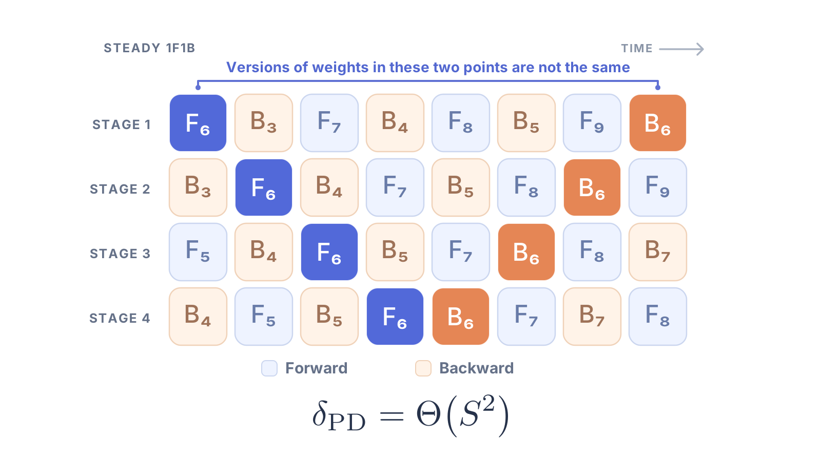
Large models are often too big to train on one accelerator. PipeDream tackles this by splitting the model into sequential stages and keeping them busy with overlapping microbatches. The pipeline runs efficiently—but it creates a striking paradox: an update can be computed from a model that never existed as one coherent parameter vector. Each stage reuses the weights that a microbatch saw during its forward pass, but that microbatch reaches different stages at different moments. By the time backpropagation returns, its stage-local snapshots belong to several points in the training history.
This project asks an optimization question about that schedule: how do PipeDream’s stale weights affect convergence, and how does their impact scale with pipeline depth?
In joint work with Peter Richtárik, we introduced Randomized PipeDream (RPD), a mathematical model that keeps PipeDream’s stage-wise staleness while replacing the exact schedule with randomized block updates. That simplification makes the mechanism analyzable. In the resulting preprint, we give the first clean nonconvex convergence guarantee for a randomized PipeDream-style method and derive how delay grows under the deterministic schedule. The analysis also points to LocalSGD as an alternative: it avoids this particular stale-read mechanism, but pays for periodic synchronization and replica drift.
Why pipeline parallelism has bubbles
A large neural network is already a chain of computational blocks. Pipeline parallelism splits that chain into ordered stages, places each stage on a different accelerator, and sends activations forward and gradients backward through them. This solves a memory problem: no single device needs to hold the entire model.
With only one microbatch in flight, however, the computation follows a strict dependency chain. Stage 2 cannot begin until stage 1 produces an activation, and the backward pass cannot begin until the final stage produces the loss. In the idealized four-stage schedule below, only one GPU works at a time, leaving three quarters of the available device-time idle.
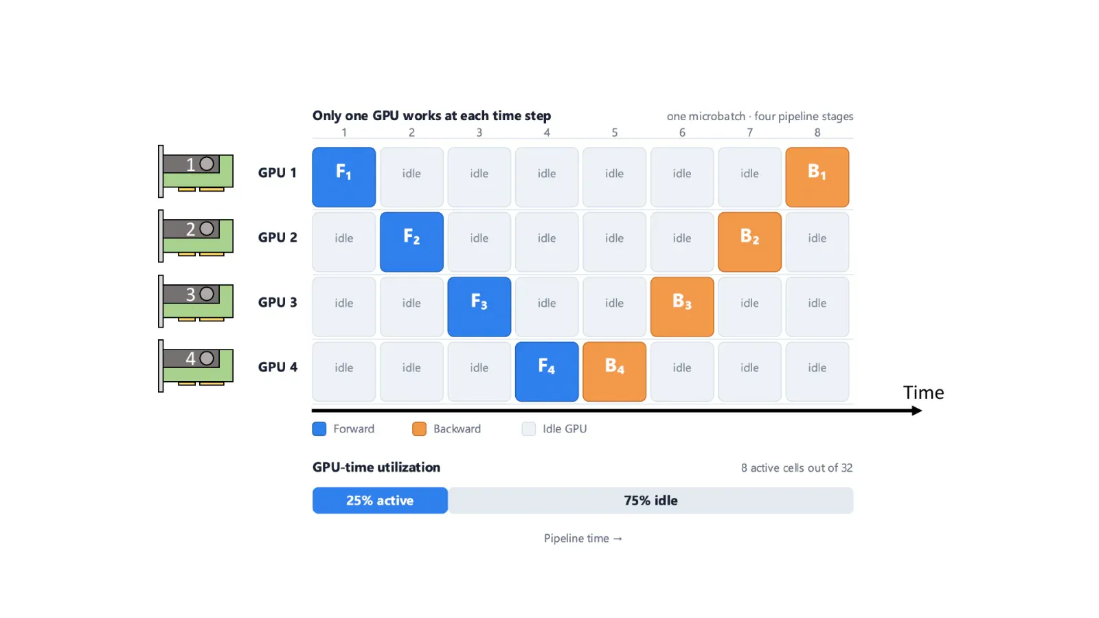
Real hardware also pays for communication, stage imbalance, kernel execution, and framework overhead. The 25% figure is therefore not a universal utilization formula; it isolates the bubble created by the forward/backward dependency chain.
PipeDream fills the bubbles—but creates stale weights
PipeDream fills much of the bubble by admitting new microbatches before older ones have finished. After startup, each stage alternates between one forward and one backward operation, a schedule known as 1F1B. Under the same equal-cost model, the steady region can be fully occupied. The schedule turns idle time into throughput.
It also changes which parameters are used to compute a gradient.
Suppose a microbatch performs its forward operation on stage 1. PipeDream saves that stage’s parameter version and reuses it when the microbatch eventually returns for the backward operation. This mechanism, called weight stashing, preserves forward/backward consistency within the stage.
But many other backward operations update the pipeline while the microbatch is in flight. The microbatch also visited each stage at a different time. Its gradient is therefore not naturally associated with one old global checkpoint; it is associated with a mixture of historical stage blocks.
To measure this precisely, let count individual backward block updates anywhere in the pipeline, rather than pipeline clock ticks. In a four-stage 1F1B simulation, the exact delays settle into a periodic pattern after warm-up:
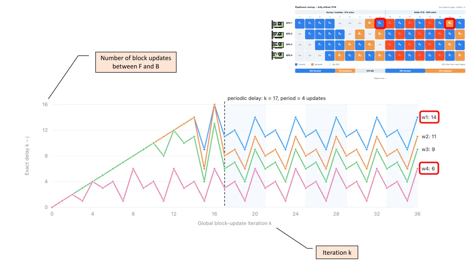
These delays are not random accidents. They are determined by the forward/backward geometry of the pipeline, unlike a generic asynchronous system in which any worker may return at any time.
How one gradient can mix several versions of the model
To describe that mixed model mathematically, start from the finite-sum objective
and split the model into the same blocks used by the pipeline:
Let be the current model after block updates. For each stage , the index records the earlier global iteration from which the stale read takes that stage’s parameters. The gradient is evaluated at
The essential point is that need not equal any past full iterate . It can take stage 1 from one moment, stage 2 from another, and so on. We assume only that every block is at most global block updates old:
This mixed model assembled from different moments in history is the part of PipeDream that RPD preserves.
Randomized PipeDream keeps the staleness, not the schedule
Exact PipeDream ties together which stage runs, which microbatch it handles, and which historical weights it sees. That makes the deterministic 1F1B timeline difficult to analyze. RPD keeps the mixed stale model but replaces this coupled schedule with a simpler randomized update.
At update , RPD first selects a bounded delay vector and forms . Given that stale model, it samples a stage and mini-batch uniformly, then updates only the selected block:
while every other block remains unchanged.
The delays themselves do not need to be uniformly random; they may depend on the history. What matters is that they are fixed before the current stage/mini-batch draw, bounded by , and followed by a conditionally uniform stage/mini-batch sample.
RPD is a lens for analysis, not a scheduler intended to run on hardware. Deterministic PipeDream does not sample its stages and microbatches uniformly. The connection back to the real system comes from deriving the delay scale produced by its actual scheduling rule.
What we can prove about RPD
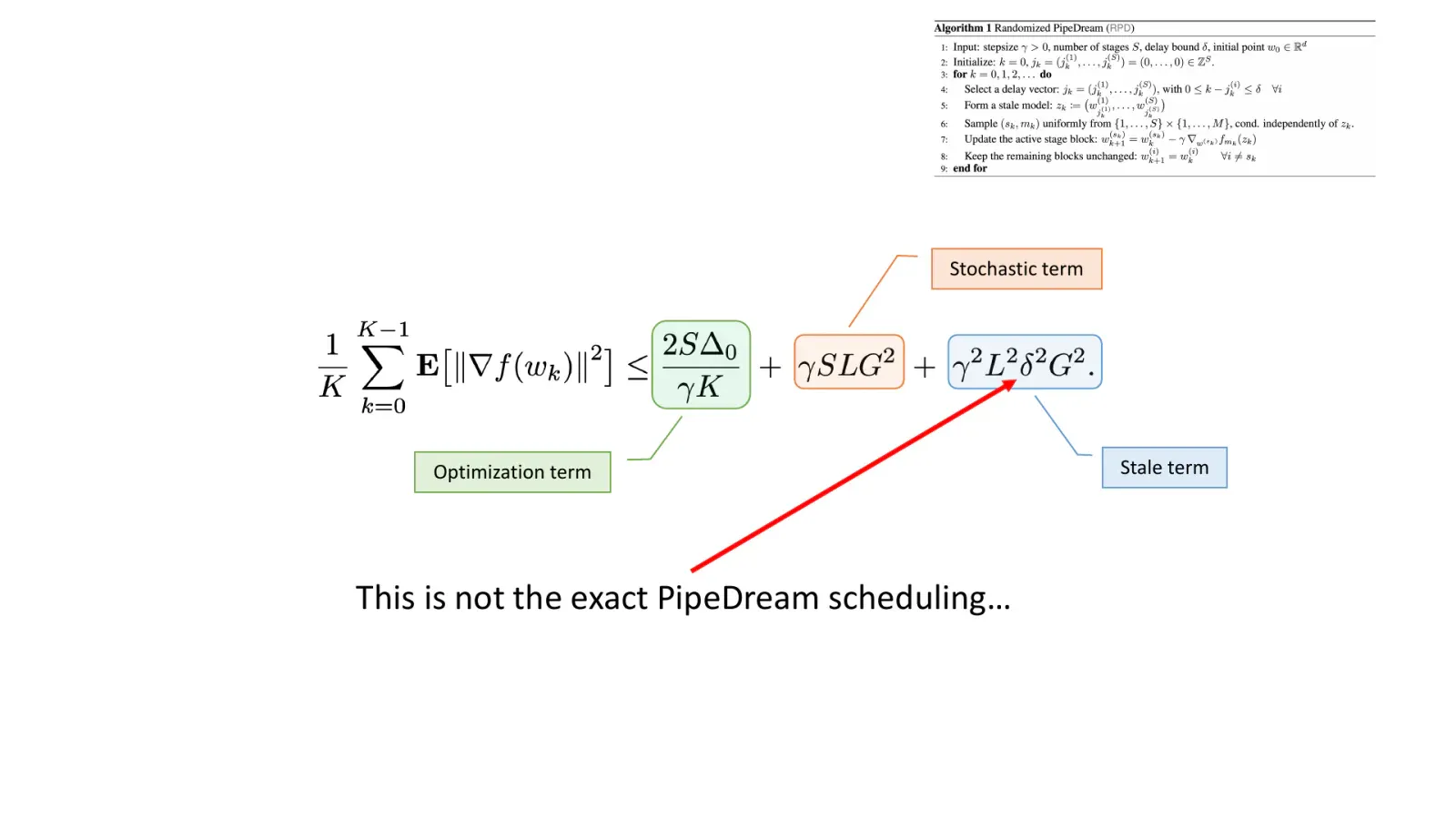
Suppose is lower bounded and -smooth, the component block gradients along the stale trajectory are bounded by , the delay is at most , and . If , then after block updates RPD satisfies
Each term tells a different part of the story:
- is the optimization term; it shrinks with the update budget.
- is the stochastic single-block update term.
- is the stale-read term. Its quadratic dependence on determines how pipeline depth enters the result.
Two observations do most of the work in the proof. First, uniform stage/mini-batch sampling makes the selected block update an unbiased full-gradient direction at , up to the factor . Second, at most intervening updates of length at most imply
Smoothness turns that parameter discrepancy into a gradient discrepancy; squaring it produces the characteristic term.
With the tuned step size
the rate becomes
A small average squared gradient norm means that the iterates are close to first-order stationarity on average. It does not imply that RPD reaches a global optimum of a nonconvex objective.
PipeDream’s delay grows quadratically with pipeline depth
We can now ask what value of corresponds to deterministic PipeDream. In steady-state 1F1B, take a stage-1 forward event and the matching stage-1 backward event. A microbatch must traverse the remaining stages and return, spanning roughly pipeline slots. Every backward block update during that round trip advances the global history, so the delay grows with the area of the intervening schedule:
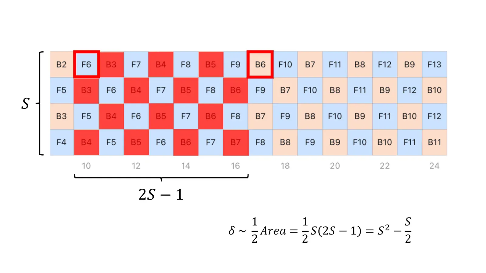
Using the paper’s convention for ordering updates within each pipeline slot, the steady-state delay is
For even , the expression is exact:
So four stages give a worst delay of block updates, matching the earlier trace, while eight stages give .
Substituting into the RPD theorem makes the raw stale-read contribution scale as . With the tuned step size, the RPD proxy for PipeDream has the form
The theory exposes a tension: deeper pipelines create more parallel work, but their gradients can be built from increasingly old stage weights.
Does RPD behave like PipeDream?
The abstraction is only useful if it retains something important about the original method. As a sanity check, we compare a deterministic PipeDream simulation with RPD on a controlled random quadratic objective.
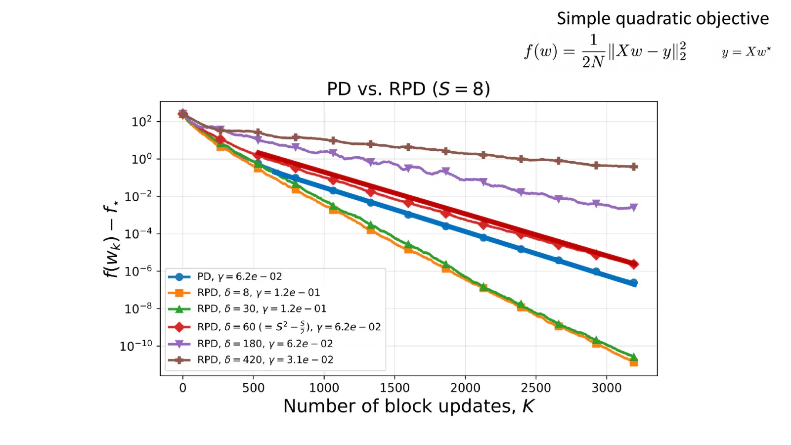
This experiment does not show that RPD reproduces every PipeDream trajectory. It supports the narrower claim that the abstraction captures an important stale-weight effect in this controlled setting.
Our proposed alternative: stage-distributed LocalSGD
The scaling law led us to propose a different way to keep the pipeline busy: apply LocalSGD across several complete model trajectories. Instead of letting one trajectory accumulate cross-stage staleness, the system maintains replicas. Each replica performs local SGD steps, after which the corresponding stage blocks are averaged:
The replicas are partitioned across the same pipeline stages and interleaved through the schedule. More trajectories provide independent work that can occupy otherwise empty slots:
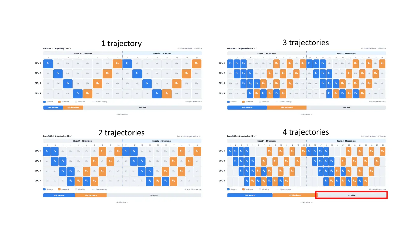
The synchronization period controls the trade-off:
- With small , replicas stay close, but frequent averaging creates more fill-and-drain bubbles.
- With large , synchronization happens less often and utilization improves, but replicas drift farther apart before averaging.
This removes PipeDream-style cross-stage staleness, but not every source of delay or error. It also requires memory for logical model copies. The experiments use to keep the pipeline highly utilized, and their optimization/time comparisons do not count this extra memory as a separate resource cost.
Compare failure modes, not universal winners
To compare the theories under a common block-update budget, let be the number of logical local steps per replica. Since each step updates all blocks for each of replicas,
With , the tuned LocalSGD guarantee becomes
The two theories expose different weaknesses:
| Model | Main systems benefit | Main optimization penalty | Additional systems cost |
|---|---|---|---|
| RPD proxy for PD | Keeps the 1F1B pipeline busy | Cross-stage stale reads; term | Startup/drain and weight stashing |
| Stage-distributed LocalSGD | Independent trajectories fill idle slots | Replica drift; term | Synchronization bubbles and logical model copies |
The guarantees also measure different quantities. RPD averages gradient norms along one stale block-update trajectory, while LocalSGD evaluates the averaged model . A shared block-update budget makes the comparison informative, but these are not identical guarantees and neither proves that one schedule always wins.
The experiments confirm that neither method wins everywhere:
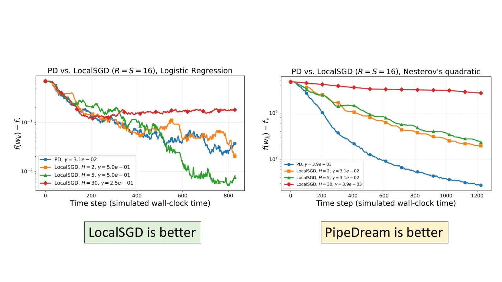
The paper also reports an 11.1M-parameter NanoChat-style Tiny Shakespeare experiment in which tuned PipeDream reaches the lower training loss. That result applies to this training setup; it is not a claim about downstream quality or generalization. Across the experiments, the outcome depends on the objective, gradient noise, stage count, memory budget, and synchronization period.
What the theory reveals
RPD is not meant to replace PipeDream’s scheduler. It gives us a way to analyze the optimization behavior that the scheduler creates:
- RPD captures the unusual model behind a PipeDream gradient: its stage blocks may come from different moments in history.
- The theorem makes delay explicit: the stale-read term depends on .
- The real scheduler supplies the scale: steady-state PipeDream has in global block-update history.
- The framework extends to other PipeDream-style methods: for any variant with bounded block-wise stale weights, derive the delay bound induced by its schedule and substitute it into the RPD rate . Under the same assumptions, this converts the method’s scheduling geometry into a convergence-rate bound.
- LocalSGD offers a different bargain: it removes this stale-version mechanism but introduces synchronization and replica drift.
The practical question is therefore not, “Which method always wins?” It is:
Which cost can this training problem afford—idle time, stale weights, or replica drift?
That is the trade-off exposed by the theory and experiments.
For the complete theory and experimental details, read the paper and explore the open-source repository.
Citation
@article{ilin2026demystifying,
  title={Demystifying Pipeline Parallelism: First Theory for PipeDream},
  author={Ilin, Ivan and Richt{\'a}rik, Peter},
  journal={arXiv preprint arXiv:2606.03498},
  year={2026}
}